Fuel Price Analysis in QLD

Introduction

This project analyzes Queensland fuel price data to identify pricing trends across fuel types and time The analysis was conducted using R programming.

Importing Data and necessary libraries

#Importing data
fueldata <- read.csv("data/qld_fuel.csv")

#Loading packages
library(dplyr)

Attaching package: 'dplyr'

The following objects are masked from 'package:stats':

    filter, lag

The following objects are masked from 'package:base':

    intersect, setdiff, setequal, union

library(lubridate)

Attaching package: 'lubridate'

The following objects are masked from 'package:base':

    date, intersect, setdiff, union

library(ggplot2)
library(plotly)

Attaching package: 'plotly'

The following object is masked from 'package:ggplot2':

    last_plot

The following object is masked from 'package:stats':

    filter

The following object is masked from 'package:graphics':

    layout

library(ggpubr)

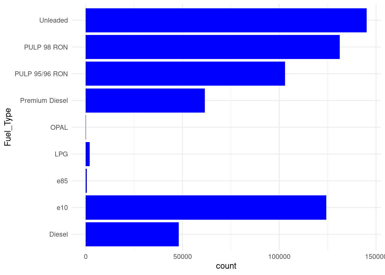
Overview of Fuel Types and total number of transcations

fueldata <- fueldata |> 
select(-X, -X_id) #removing X and X_id column

#converting date from str to date
date <- fueldata$TransactionDateutc
date <- ymd_hms(date)
#unique Fueltypes or types of fuels
unique(fueldata$Fuel_Type)

[1] "Diesel"         "PULP 98 RON"    "Unleaded"       "e10"           
[5] "LPG"            "Premium Diesel" "PULP 95/96 RON" "e85"           
[9] "OPAL"          

ggplot(fueldata,
       aes(y= Fuel_Type))+
geom_bar(fill = "blue")+theme_minimal()

Top 5 Fuel Brands

Available Fuel Brands in QLD and the Top 5 fuel brands with the highest number of transcations over the year are.

#fuel Companies

unique(fueldata$Site_Brand)

 [1] "Liberty"              "BP"                   "7 Eleven"            
 [4] "EG Ampol"             "Coles Express"        "Ampol"               
 [7] "Caltex"               "Freedom Fuels"        "Metro Fuel"          
[10] "Pearl Energy"         "Independent"          "Shell"               
[13] "Puma Energy"          "United"               "Pacific Petroleum"   
[16] "Mobil"                "Pacific Fuel Solutio" "Matilda"             
[19] "Enhance"              "Astron"               "Lowes"               
[22] "IOR Petroleum"        "Unknown"              "Choice"              
[25] "Costco"              

#Top 5 brands 
top5 <- fueldata |> 
count(Site_Brand, sort= TRUE) |> 
 head(n = 5)

print(top5)

     Site_Brand      n
1      7 Eleven 118040
2         Ampol 105750
3            BP  84121
4 Coles Express  71882
5      EG Ampol  62774

ggplot(top5,aes(x=Site_Brand, y=n))+geom_col(fill= "light green")+theme_minimal()

Summary of Fuel Price

summary(fueldata$Price)

   Min. 1st Qu.  Median    Mean 3rd Qu.    Max. 
      1    1869    1999    2005    2139    9000 

mean(fueldata$Price)

[1] 2005.467

median(fueldata$Price)

[1] 1999

sd(fueldata$Price)

[1] 203.584

#Histogram of data
ggplot(fueldata,
aes(Price))+
geom_histogram(fill="orange", bins=40)+
theme_minimal()

Fuel types and Prices

All fuel types does not cost similar price at any given time as many differnt factors account for the pricing. For example, LPG is one of cheapest fuel while PULP 98 is the expensive fuel type.

Average pricing of all fuel types.

#Fuel prices by fuel type
ggplot(fueldata,
aes(x=Fuel_Type, y=Price,
fill=Fuel_Type))+
geom_boxplot()+
theme_minimal()+
coord_flip() 

Trend of FUEL Price by month

# monthly prices 
fueldata <- fueldata |>  # update data with the new column month
  mutate(month = month(date))

monthly <- fueldata |> 
  group_by(month, Fuel_Type, colour=Fuel_Type) |> 
  summarise(
AveragePrice=mean(Price)
)

`summarise()` has grouped output by 'month', 'Fuel_Type'. You can override
using the `.groups` argument.

ggplot(monthly,
aes(month,
AveragePrice,
))+
 geom_point(aes(colour=Fuel_Type))+
    geom_smooth()+
    theme_classic()

`geom_smooth()` using method = 'loess' and formula = 'y ~ x'

Making interactive

my_plot <- ggplot(monthly,
aes(month,
AveragePrice,
colour= Fuel_Type,
frame= month))+
#geom_line(color="blue")+
geom_point()+
theme_minimal()

ggplotly(my_plot)